Part II · Advanced topics · Chapter 3

Clustering

Clustering asks Graphica to find groups in your data rather than being told what they are. The result arrives as a new computed variable you can encode like any other — usually on Color, so the groups it found become visible.

Two sources

Calc clustering on decides what the grouping is computed from, and the two options answer different questions.

Source	Groups by	Use when
Links	Connection. Nodes that link to each other more than to the rest of the graph.	You have network data. This is the default.
Variables	Similarity. Rows whose values on the variables you choose resemble each other.	You have an ordinary dataset and want to know which rows behave alike.

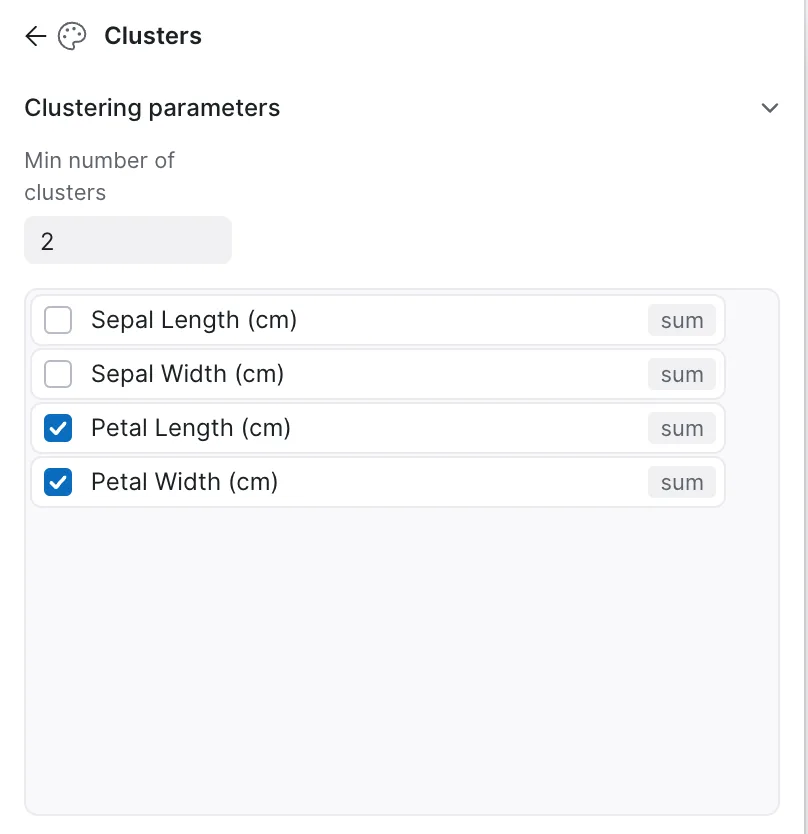
The choice only exists on network data: on an ordinary dataset there are no links to cluster on, so Calc clustering on does not appear and Graphica goes straight to variables. With Variables in effect, a checklist appears and you pick which columns take part. That choice is the analysis: clustering on population and area finds groups of similar size, clustering on literacy and income finds groups of similar development, and the two have nothing to do with each other. Choose the variables that correspond to the question you are asking, not all of them.

Min number of clusters sets the floor — six by default. It is a lower bound rather than an exact count; the algorithm may find more if the structure warrants it.

The settings of the Clusters variable on Color, under Clustering parameters: Min number of clusters set to 2, and a checklist of the dataset's numeric columns — Sepal Length and Sepal Width unticked, Petal Length and Petal Width ticked, each with a sum badge. — **Figure 1** — Clustering on chosen variables. On a dataset without links there is no source to pick; the tick boxes decide what "similar" means.

Using the result

The clusters arrive as a computed variable, listed with the others under Computed variables. From there it is an ordinary categorical column:

On Color — the standard move. Groups become visible in whatever chart you already had.
On Small Multiples — one panel per cluster, for looking at each group's internal shape.
On Unit — one mark per cluster, aggregating each group into a single summary.
On Subdivision — to see how clusters compose some other grouping.

One thing it cannot do

The clusters variable cannot go on Filters; you will get This computed variable cannot be used as a filter.

The reason is circularity: clusters are computed from the data being drawn, so filtering by them would change the input that produced them. To narrow the chart, filter on the underlying variables and let the clustering recompute.

Reading the result honestly

Clustering always returns clusters. It has no way of telling you that your data has no group structure — it will partition uniform noise into six tidy groups and colour them convincingly. That makes a few habits worth having.

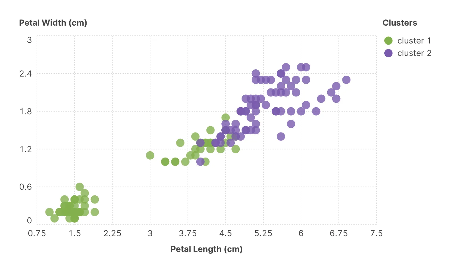
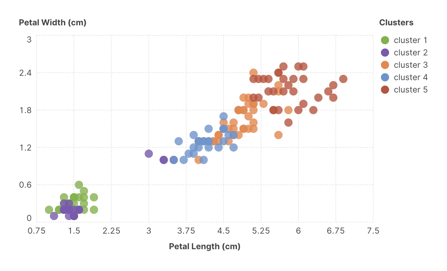
Vary the minimum and watch. Groups that survive a change in the cluster count are telling you about the data. Groups that reshuffle completely were telling you about the parameter.
Check the boundaries. Colour by cluster and look at where two clusters meet. If there is a visible gap, the split is real; if they blend, the line is arbitrary and should be described as such.
Watch the units. Clustering on variables measures distance across them, so a column in millions will dominate one measured from 0 to 1. If the variables are on wildly different scales, normalize them into computed columns first — see the Calc and Percentage options in Data types.
Name what you found. Cluster 3 means nothing to a reader. Once you understand what a group has in common, say so in the legend title or the footer.

A cluster is a hypothesis

The output is a suggestion about structure, produced by an algorithm that was given no context. Presented without qualification, coloured groups read as established fact — readers assume someone verified them.

Treat a clustering as something to investigate and then explain, not as a finding in itself.

Iris flowers plotted by petal length and width, colored by clusters computed from all four measurements with Min number of clusters at 2: one group holds the small-petalled setosa flowers and a few others, the second holds the rest. — **Figure 2** — The same data at two cluster counts. The groups that survive are the ones worth talking about.

The same plot with Min number of clusters at 5: the large group splits into three overlapping bands along the diagonal, and the setosa group splits into two subgroups mixed together in the same corner. — **Figure 2** — The same data at two cluster counts. The groups that survive are the ones worth talking about.

Where to go next

Clustering finds groups. Reference lines and regression analysis finds trends — the other way of drawing a conclusion on top of your marks.